This script depicts the specific and in-depth characterization of the clusters related to the disease-associated microglia (DAM) signature, including gene markers, gene ontology, gene set enrichment anaysis, and transcription factor enrichment, related to Figure 3.
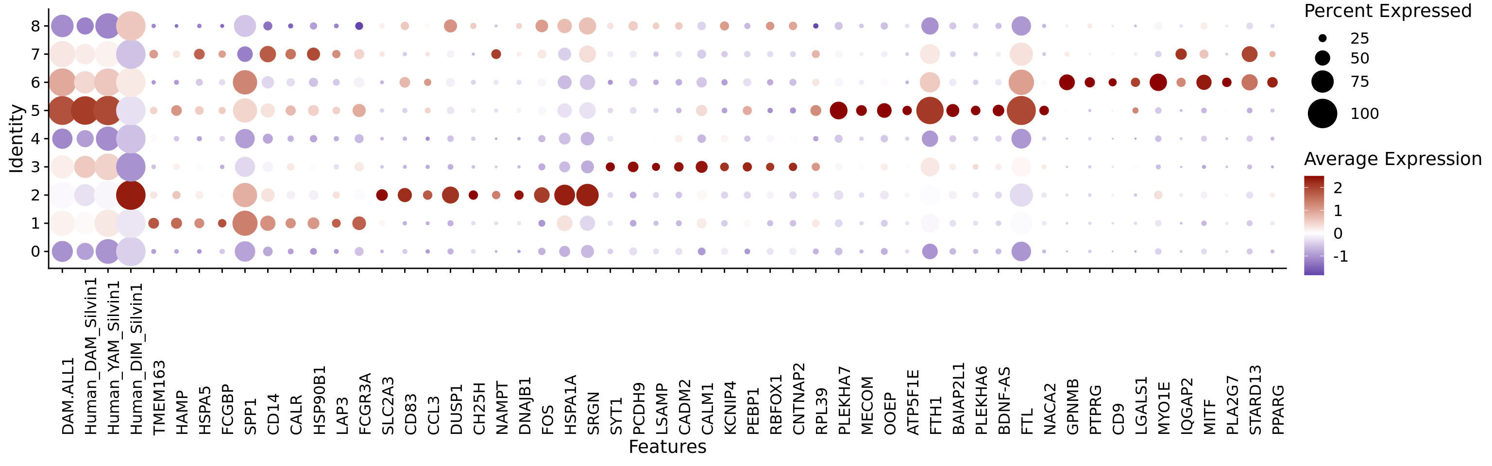
Based on the Module Score expression of the original DAM signature from Keren-Shaul et al (2017) and the more recent DAM, DIM (disease-inflammatory macrophage) and YAM (youth-associated microglia) from Silvin et al (2022), we determined clusters 1, 2, 3, 5 and 6 as DAM-related. In addition to the mentioned Module Scores, we represented the expression of the top 10 significant markers for each cluster. The used sigantures are included at the “Genesets_literature” file in this repository (“Support data”).
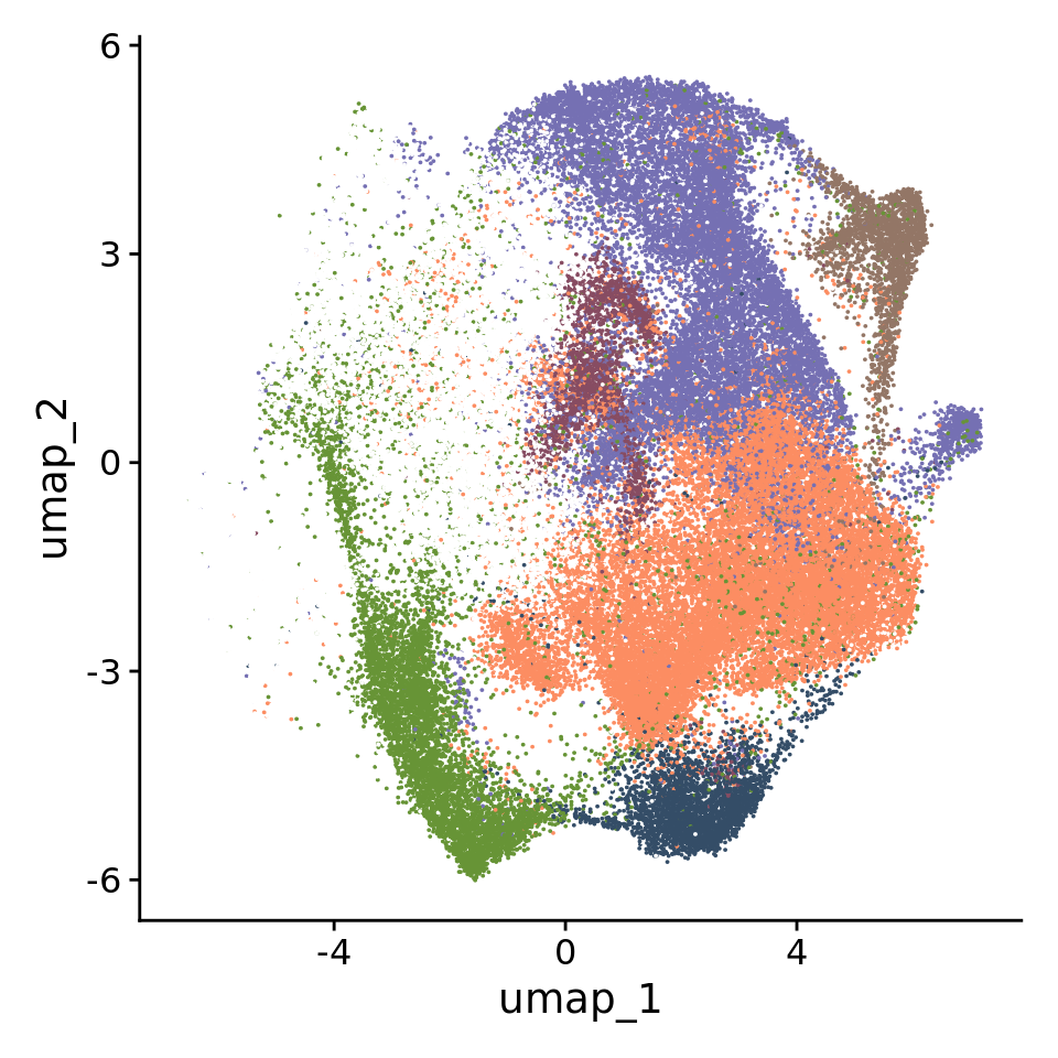
The representation of the HuMicA object was edited to depict only the five populations enriched for the DAM signature, namely clusters 1 (Inflam.DAM), 2 (DIMs), 3 (Ribo.DAM1), 5 (Ribo.DAM2) and 6 (Lipo.DAM). Of note, cluster 7 (Border-Associated Macrophages) ara also represented, to support the potential macrophagic nature of the DIMs, based on the proximity of both populations in the UMAP. This annotation was based on the previous enrichment presented in Figure 1F, the above DotPlot and the enrichment analysis that will be presented bellow.
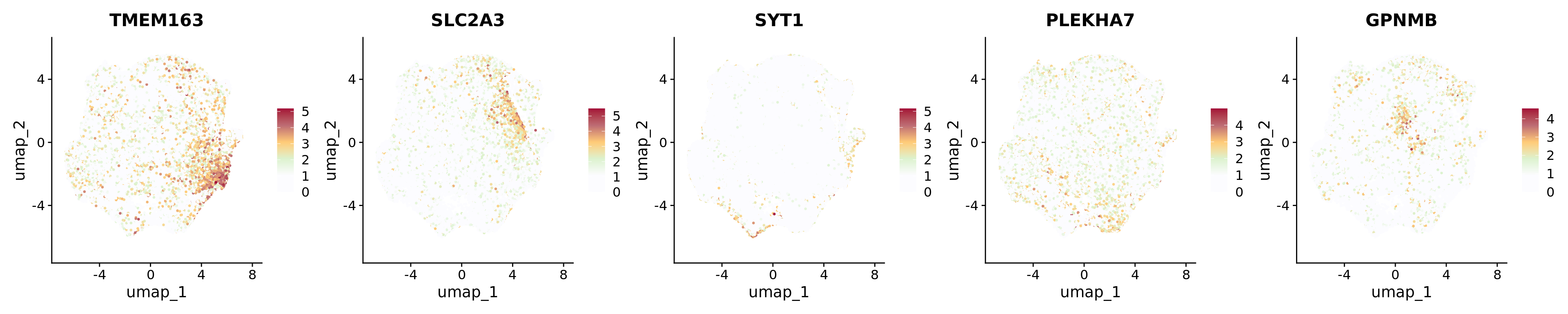
The most prominent markers of each cluster were represented separately in Feature plots: TMEM163 for Inflam.DAM; SLC2A3 for DIMs; SYT1 for Ribo.DAM1; PLEKHA7 for Ribo.DAM2; and GPNMB for Lipo.DAM (related to Supplementary Figure 7A).
Humica <-SetIdent(Humica, value = Humica@meta.data$integrated_snn_res.0.2)DefaultAssay(Humica)<-"RNA"Humica <-NormalizeData(Humica)FeaturePlot(Humica, features =c("TMEM163","SLC2A3","SYT1","PLEKHA7","GPNMB"), ncol=5,label = F, repel =TRUE,pt.size =0.5) &scale_colour_gradientn(colours =c("#FCFCFF","#FCFCFF","#DCF2CE","#FFCB77","#BD6B73","#A30B37"))
Scale for colour is already present.
Adding another scale for colour, which will replace the existing scale.
Scale for colour is already present.
Adding another scale for colour, which will replace the existing scale.
Scale for colour is already present.
Adding another scale for colour, which will replace the existing scale.
Scale for colour is already present.
Adding another scale for colour, which will replace the existing scale.
Scale for colour is already present.
Adding another scale for colour, which will replace the existing scale.
Gene ontology
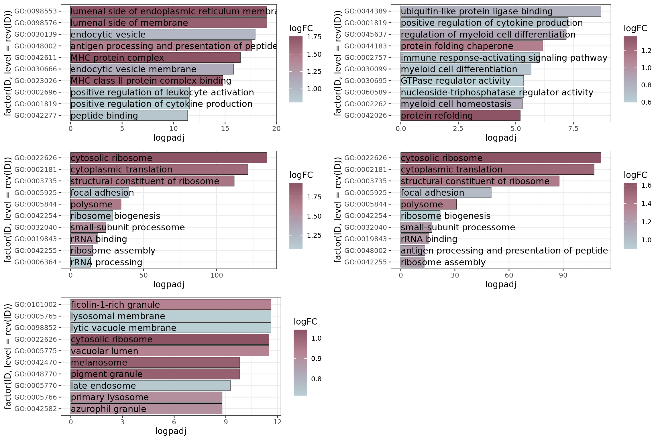
Gene ontology (GO) was calculated with the enrichGO function from clusterProfiler.
Barplots
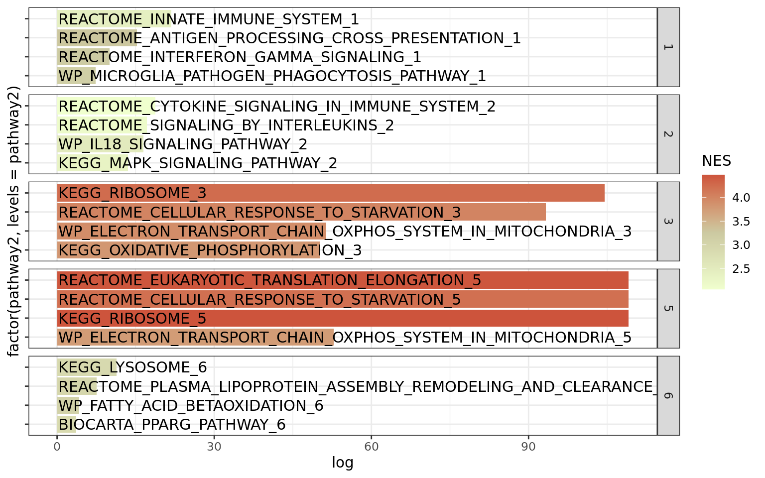
The top 10 significant GO terms for each of the homeostatic clusters were represented in barplots to provide a broader insight on the GO enrichment (related to Supplementary Figure 7B). GO was recalculated and edited to obtain the Fold Change of enrichment.
Warning: Using `size` aesthetic for lines was deprecated in ggplot2 3.4.0.
ℹ Please use `linewidth` instead.
do.call(grid.arrange,p)
Gene set enrichment analysis (GSEA)
GSEA analysis was performed using as reference all genesets from msigdbr for the “C2” category of “Homo sapiens”. The results from FindAllMarkers with a less significant cutoff were used as cutoff. This intends to account for the broad spectrum of differential expression and not only the significant differentially expressed markers (only.pos = F, min.pct = 0.1, logfc.threshold = 0.0, test.use = “MAST”). Of note, both up and downregulated markers were considered at “Humica.markers”. The avg_log2FC and the p_val_adj were used for ranking.
A list of terms of interested were selected from the results output. The results are presented as a function of the Normalized Enrichment Score (NES) and the negative of the log of the adjusted p value.
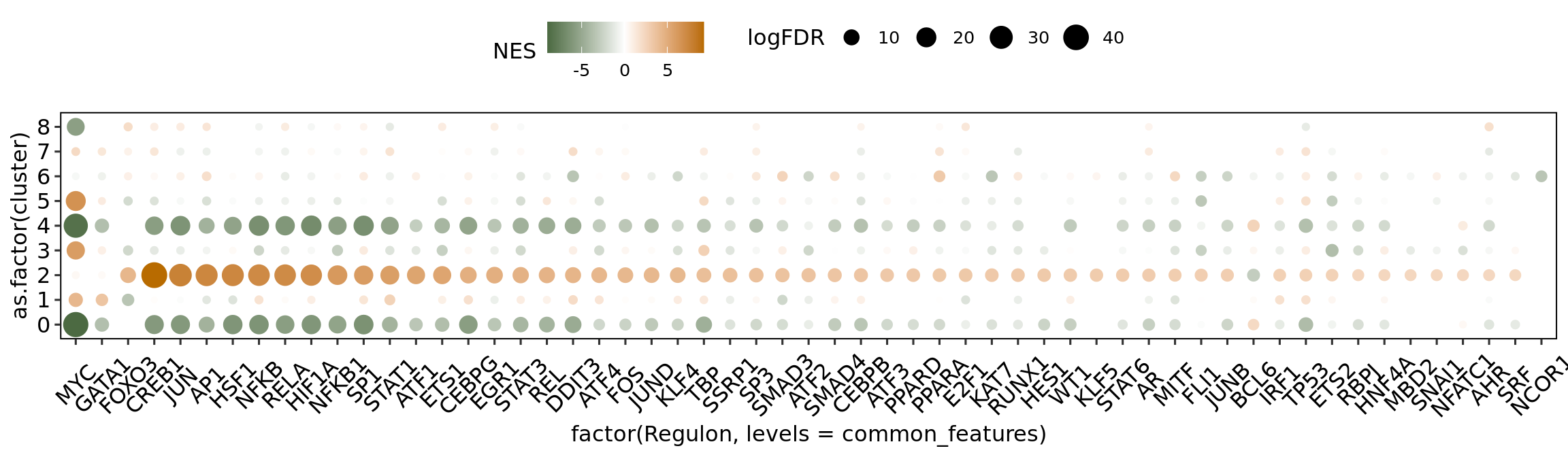
The collection of transcription factors (TFs) and their target genes was obtained from the CollecTRI repository from decoupleR. The enrichment analysis was performed using the viper package. The Humica.markers file correspond to the broad spectrum differential expression output, mentioned in the “Characterization of the HuMicA” script of this repository. The following represents the loop for the calculation of TF enrichment in all nine clusters.
#Create the regulon from the CollecTRI repository in the appropriate format for viper.net <- decoupleR::get_collectri(organism='human', split_complexes=FALSE)## create regulon for viper# Function to create named tfmode and add likelihoodcreate_named_tfmode <-function(df) {# Ensure tfmode is numeric tfmode_named <-setNames(as.numeric(df$mor), df$target) likelihood_vector <-rep(1, length(tfmode_named)) # Assuming constant likelihood of 1list(tfmode = tfmode_named, likelihood = likelihood_vector)}# Group by source and apply the transformationsource_target_list <- net %>%group_by(source) %>%summarise(tfmode =list(setNames(as.numeric(mor), target)),likelihood =list(rep(1, n())) ) %>%deframe()
Warning: `x` must be a one- or two-column data frame in `deframe()`.
The plot depicts the enrichment for all clusters in the HuMicA but only considers the significant TFs for the three homeostatic clusters is considered for representation. The statistically significant TFs were considered for an adj p value (FDR) < 0.05.